The client
Five plants, one order queue, no arbitration
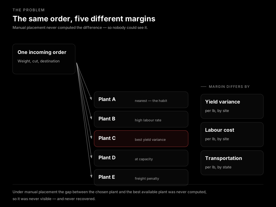
A pork producer running five processing facilities. Every incoming order has to be assigned to one of them.
And that assignment determines the margin on the order — which is the part nobody was computing.
The challenge
The assignment was habit, not arithmetic
The process for placing orders was manual, and manual assignment across five plants reliably produces suboptimal allocation. A person cannot weigh yield variance against labour rate against freight cost against available capacity, per order, at volume. So they use proximity, and a feel for which plant is busy.
What the manual process could not see
The three stated goals were straightforward: maximise profit by optimising placement, improve resource utilisation across facilities, and reduce operational cost in processing and fulfilment.
But the real problem was epistemic before it was economic. You cannot recover a cost you have never measured, and nobody could say what a badly-placed order had cost.
Constraints
What we had to design around
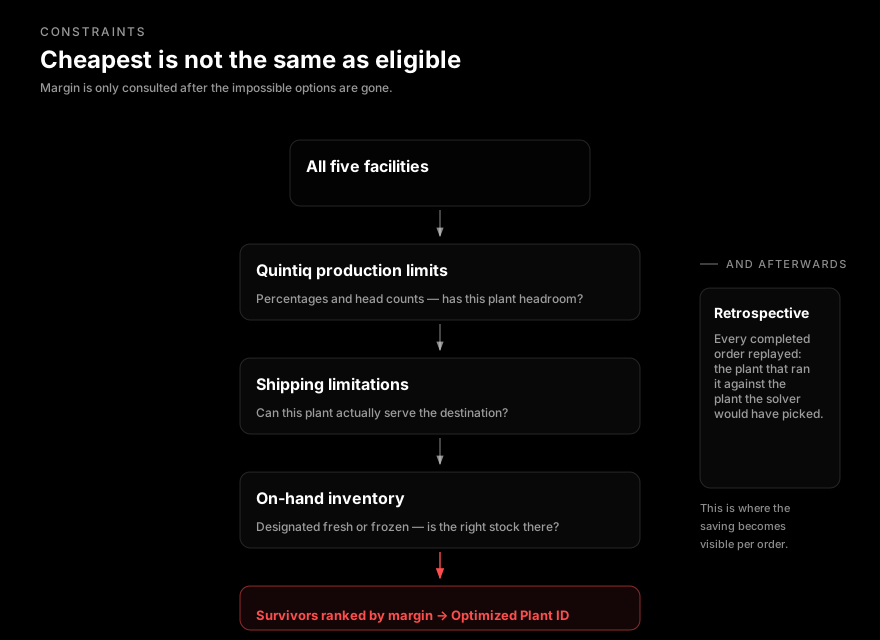
- CapacityQuintiq production limits, expressed both as percentages and as head counts. A plant with the best margin and no headroom is not an option.
- ShippingRoute limitations between plants and destinations. Some plants simply cannot serve some places, whatever the arithmetic says.
- InventoryOn-hand stock, with fresh and frozen designated separately — so availability is two questions, not one.
- GeographyFreight cost aggregates by state, so the cost surface is not uniform and the nearest plant is not reliably the cheapest.
The last one is why proximity is a bad heuristic rather than a rough-but-fine one. Freight aggregates by state, so the nearest plant is not reliably the cheapest — and the error is not random, it is systematic in whichever direction the freight table happens to lean.
Our approach
Make the trade-off explicit and computable
Three cost components, each normalised per pound and scaled by the order’s net weight.
The objective, as the client defined it
Combined into the expression the solver optimises, written the way the client already wrote it:
Total Cost = Yield Variance − Labor Cost − Transportation Cost
The optimised plant is the one with the greatest margin increase across those three, filtered to the lowest cost available with capacity.
The solution
A recommendation, and a retrospective
- Decompose the cost — Three components, each derived per pound and scaled by the order’s net weight: yield variance, labour cost, and transportation with freight aggregated by state.
- Filter for eligibility — Candidate plants are removed by Quintiq production limits, then shipping limitations, then on-hand fresh/frozen inventory — before margin is consulted at all.
- Rank the survivors — Whatever is left is ranked by margin, and the highest becomes the Optimized Plant ID for that order.
- Replay the history — Completed orders are re-scored: the plant that actually processed each one against the plant the solver would have chosen.
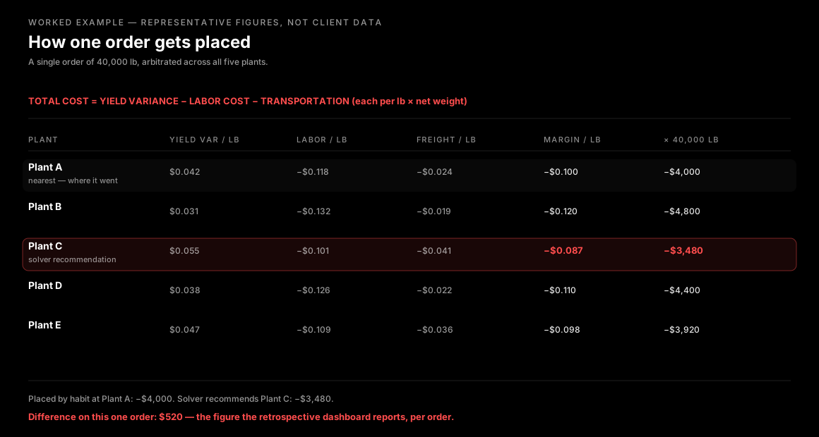
The retrospective is the half that made it adoptable. The dashboard replays previous orders, comparing the Plant ID that actually processed each one against the Optimized Plant ID the solver would have recommended.
Savings left on the table become visible per order — which is a far more persuasive artifact than a forecast, because it is about orders the planner remembers.
Responsible by design
Four rules that keep a solver trusted
Eligible first
Margin is only consulted after the impossible options are gone.
A recommendation the plant cannot physically fulfil is worse than no recommendation — it costs the planner their trust in the tool.
Show the working
Every recommendation decomposes into its three components.
A planner who can see that freight, not labour, is what moved the answer can argue with it — and correct it when the freight table is stale.
Prove it backwards
The dashboard scores the past, not the future.
A forecast asks to be believed. A replay of last quarter’s orders against what they would have earned elsewhere does not.
Recommend, do not place
The solver proposes an Optimized Plant ID. A person still places the order.
Nothing in the constraint model knows about a customer relationship or a maintenance window someone has in their head.
The third one is the load-bearing rule here. Optimisation tools are usually sold on a projection, and planners have learned to discount projections. Scoring the past — orders they remember placing, against what those orders would have earned elsewhere — is an argument they can check.
Results
What the solver produces
- Every order is now arbitrated across all five plants, against three cost components and three constraint families — rather than assigned by proximity and habit.
- The margin gap became visible per order, which is the change that matters: the difference between where an order went and where it should have gone was previously never computed at all.
- The freight table stopped being invisible. Because transportation is decomposed out separately and aggregated by state, a stale freight figure now shows up as a wrong recommendation instead of quietly distorting every placement.
Beyond the numbers
What else changed
Placement stopped being a judgment call and became a decision with a receipt. That matters beyond the margin: when a planner overrides the recommendation for a reason the model does not hold — a customer relationship, a maintenance window — the override is now visible and costed rather than indistinguishable from routine.
The same decomposition also exposed the freight table as a first-class input rather than a background assumption. It had been distorting every placement quietly; now a stale figure surfaces as a recommendation someone disagrees with.
What this page does not claim. The engagement produced no published aggregate savings figure, so there is none here. The solver was built, the constraints were modelled and the retrospective dashboard quantifies the gap per order — but the total it added up to across the order book was never written down, and we are not going to estimate one after the fact. The worked example above uses representative figures to show the mechanism, not the outcome.
If your allocation decisions are made on proximity and feel
The first question is not which solver. It is whether the cost of a bad allocation is measurable at all from your historical orders — and usually it is, before anything gets built.